Data Analysis on unforgettable.me: Preprocessing Your Data
It is often the case that data needs to be preprocessed - joining different sources together, creating new variables, filtering out rows and aggregating across rows - before conducting an analysis or producing a plot. In this tutorial, we will discuss how you can use the Compute, Filter and Aggregate boxes to organize your data.
Data will typically come from multiple sources. In Demo Project (Event Segmentation Project V2), you will see data from the __App__, __IFTTTGoogleCalendar, __SEMAg5zn5ggo_B__, __USurveyDemographic__, __USurveyGeographic__, __USurveyHealth__, __USurveyLanguages__, __USurveyRelationships__, USurveySocioEconomic__, __USurveyTimeUse__, and __USurveyWork__ data streams. When you are conducting an analysis though, you most probably will select variables that come from a subset of these sources.
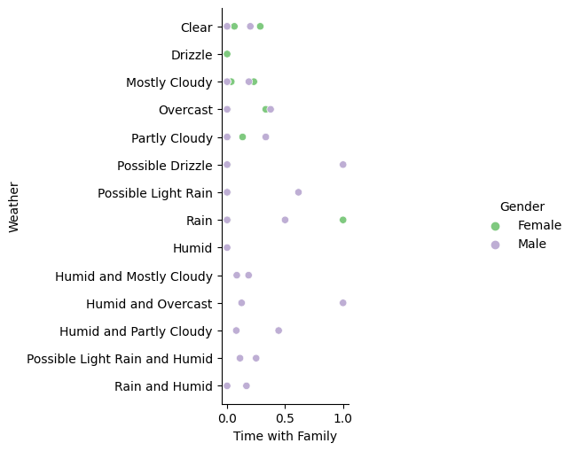
For instance, if you were interested in the relationship between weather and time spent with family as a function of gender, you might select __App__Weather, __SEMAg5zn5ggo_B__PeoplePreviousEvent1[1] and __USurveyDemographic__Gender. In this case, you have selected variables from the __App__ , __SEMAg5zn5ggo_B__ and __USurveyDemographic__ sources.
The sources you select are joined to create one big table. Only data corresponding to the same user is joined and temporal sources like __App__ and __SEMAg5zn5ggo_B__ are joined based on the nearest match on their timestamp. Temporal events will only be joined if they are within a half hour of each other.
For example, let's suppose the original sources contained the following rows:
__App__ | ||||
UserId | StartDateTime | Latitude | Weather | ... |
U1 | 8am 5th May 2021 | -37.835597 | Rain | |
U1 | 9am 5th May 2021 | -37.835594 | Rain | |
U1 | 10am 5th May 2021 | -37.835599 | Clear | |
U2 | 8am 5th May 2021 | -37.835642 | Clear | |
U2 | 9am 5th May 2021 | -37.835643 | Possible Light Rain | |
U3 | 9am 5th May 2021 | -37.835585 | Drizzle | |
__SEMAg5zn5ggo_B__ | ||||
UserId | StartDateTime | PeoplePreviousEvent1 | ActivityPreviousEvent1 | ... |
U1 | 7:35am 5th May 2021 | 1 | 1 | |
U1 | 9:12am 5th May 2021 | 0 | 0 | |
U2 | 7:50am 5th May 2021 | 1 | 0 | |
U2 | 8:20am 5th May 2021 | 0 | 0 | |
U2 | 10:16am 5th May 2021 | 0 | 0 | |
U3 | 9:12am 5th May 2021 | 0 | 1 | |
__USurveyDemographic__ | ||||
UserId | StartDateTime | Education | Gender | ... |
U1 | 11:15am 8th January 2019 | Graduate Degree (MA/MSc/MPhil/other) | Male | |
U1 | 1pm 19th December 2020 | Graduate Degree (MA/MSc/MPhil/other) | Trans Female/Trans Woman | |
U2 | 10:01pm 17th April 2021 | Undergraduate (BA/BSc/Other) | Female | |
U3 | 7:01pm 2nd February 2018 | Undergraduate (BA/BSc/Other) | Male | |
The resulting table would be:
UserId | __App__Weather | __SEMAg5zn5ggo_B__PeoplePreviousEvent1 | __USurveyDemographic__Gender |
U1 | Rain | 1 | Trans Female/Trans Woman |
U1 | Rain | 0 | Trans Female/Trans Woman |
U2 | Clear | 1 | Female |
U3 | Drizzle | 0 | Male |
To see how we arrived at this result, consider the __App__ table. U1's first StartDateTime was 8am 5th May 2021. The row at 7:35am 5th May 2021 in the __SEMAg5zn5ggo_B__ table is within half an hour of this time, so we create a row for U1 with "Rain" in the weather column and 1 for the PeoplePreviousEvent1 column (indicating that U1 was with their family at this time).
U1's second StartDateTime was 9am 5th May 2021. The second row in the __SEMAg5zn5ggo_B__ table is within a half hour of this time, so we create a row for U1 with "Rain" for the weather and 0 for the PeoplePreviousEvent1 (indicating that U1 was not with their family at this time).
U1's third StartDateTime is not within a half hour of any row in the __SEMAg5zn5ggo_B__ table and so it is dropped.
U2's first StartDateTime is 8am 5th May 2021. Now we have two options to match to this row - 7:50am 5th May 2021 and 8:20am 5th May 2021 are both within a half hour. Because 7:50am 5th May 2021 is closer though, we go with that and we include "Clear" for the weather and 1 for the PeoplePreviousEvent1 (indicated that U2 was with their family at this time).
U2's second StartDateTime is 9am 5th May 2021. There are no rows in the __SEMAg5zn5ggo_B__ table for U2 within half an hour of this row, so it is dropped.
U3's only StartDateTime in the __App__ table is 9am 5th May 2021. There is a matching row in the __SEMAg5zn5ggo_B__ table, so we add Drizzle and 0 to the table.
FInally, we consider the nontemporal sources - __USurveyDemographic__ in this case. Note that although __USurveyDemographic__ is not a temporal source per se, it can still change if for instance, a participant completes a survey multiple times. In the current case, U1 has undergone a gender transition. In this case, we take the most recent values in the __USurveyDemographic__ table and join on the basis of the UserId.
This section has demonstrated how the initial table is created based on the data sources that are selected (or that appear in expressions, see below). The following sections show how new variables are created, rows are filtered and rows aggregated to form the final table on which an analysis is conducted.
Compute
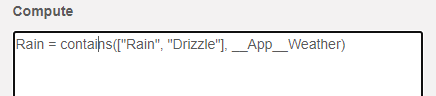
The Compute box allows you to define new variables based on the values of the other variables in a row of data. For instance, __App__Weather indicates the precipitation that occurred in each hour period. There are 17 possible values[a][b] that __App__Weather (see figure above). Let's suppose though that you would like to conduct an analysis in which you are only interested in whether it was raining or not. We can define a new variable "Rain" in the Compute box as follows:
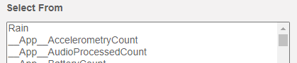
Now a new variable Rain will appear in the Select From list and you can choose to conduct subsequent analyses on this variable:
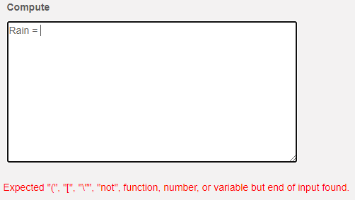
If you were entering the code on the interface, you will have noticed that a red error message appeared below the Compute box as you were typing:
The error indicates that the definition of the variable is not yet correct. The message indicates what the parser is looking for - in this case a (, [, ", function number or variable. When you complete the definition, the error will disappear.
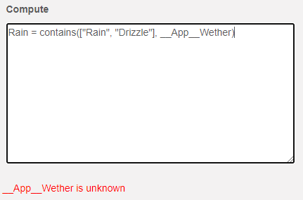
The other kind of error you can receive occurs when the definition is well-formed, but you have referenced a function or variable that the system does not know about:
In this case, we have spelt Weather incorrectly. If you correct the spelling the error will go away.
Now let's look at the code.
Rain =
indicates that we wish to create a new variable called Rain. The definition of the variable follows the = sign.
contains(["Rain", "Drizzle"], __App__Weather)
The keyword “contains” denotes a special function that takes a list of terms and a variable. If any of the terms in the list appear in the variable on each given row, the corresponding value of the new variable will be True. Otherwise, it will be False.
In this case, if the word "Rain" or the word "Drizzle" appears in __App__Weather, Rain will be True for the corresponding row. Otherwise it will be False.
Applying this code to our previous example, we would get the following table:
UserId | __App__Weather | __SEMAg5zn5ggo_B__PeoplePreviousEvent1 | __USurveyDemographic__Gender | Rain |
U1 | Rain | 1 | Trans Female/Trans Woman | True |
U1 | Rain | 0 | Trans Female/Trans Woman | True |
U2 | Clear | 1 | Female | False |
U3 | Drizzle | 0 | Male | True |
We can now select Rain as a variable in the same way we would select any other variable and use it in our analyses.
You can use the normal arithmetic operators in the expressions you create (+, -, *, /) as well as logical operators like and, or, not, >, <, ==, !=, <=, and[c] >=. For instance, you could write:
RainNorthern = Rain and (__App__Latitude > 0)
to indicate that the variable should only be True if it was running and in the northern hemisphere.
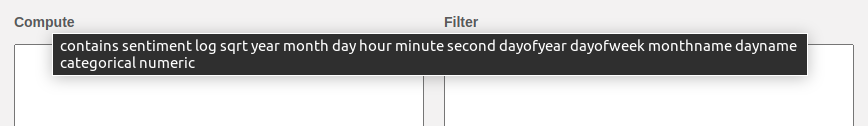
There is also a set of functions that you can employ. This set is evolving, but you can see what is available by hovering your mouse pointer over the Compute label.
Currently, the function list includes:
contains: Takes a list of terms and a text variable and indicates if any of the words in the list appears in the text. e.g. contains(["Rain", "Drizzle"], __App__Weather) returns True or False.
sentiment: Indicate sentiment of text. The NRC emotion database is used to count the number of words in the text that carries a given sentiment. The available sentiments are trust, fear, negative, sadness, anger, surprise, positive, disgust, joy or anticipation. e.g. sentiment("sadness", __UUTwitter__Text)
log: Calculate the log of the variable. e.g. log(__App__Kilometers)
sqrt: Calculate the square root of the variable. e.g. sqrt(__App__Kilometers)
year, month, day, hour, minute, second, dayofyear, dayofweek, monthname, dayname: Take a date time variable and extract a component. e.g. monthname(__App__StartDateTimeLocal) returns January, February, March, April, May, June, July, August, September, October, November or December.
categorical: convert the value to a categorical variable. e.g. month(__App__StartDateTime) would return the months as numbers, but if you want to use these as categorical values for the purposes of counting, you would need categorical(month(__App__StartDateTime)).
numeric: convert the variable to a numeric variable (or None if that is not possible).
Filter
To isolate conditions or exclude outliers, it is often useful to be able to exclude rows from the data. Adding expressions to the Filter box ensures that only rows that satisfy these conditions will be included in the data to be analyzed.
For instance, we could add:
__USurveyDemographic__Gender != "Male"
to the Filter box. Our table would then become:
UserId | __App__Weather | __SEMAg5zn5ggo_B__PeoplePreviousEvent1 | __USurveyDemographic__Gender | Rain |
U1 | Rain | 1 | Trans Female/Trans Woman | True |
U1 | Rain | 0 | Trans Female/Trans Woman | True |
U2 | Clear | 1 | Female | False |
You can also use arithmetic operators (+, -, *, /) and boolean operators (not, and, or, ==, !=, <, >, <=, >=) in your expressions as well as brackets.
Aggregate
Experience sampling data often comes at two levels - each participant will often have many GPS, microsurvey or social media posts - for example. In order to fully utilize the rich data experience sampling provides, we need to aggregate responses within individuals. The unforgettable.me analysis system groups the rows by the categorical variables in the selected set (excluding those defined in the Aggregate box) and then applies a function to the rows in each group.
For instance, if we selected the variables in our small example above, we would get the following table:
UserId | __App__Weather | __SEMAg5zn5ggo_B__PeoplePreviousEvent1 | __USurveyDemographic__Gender | Rain |
U1 | Rain | 0.5 | Trans Female/Trans Woman | True |
U2 | Clear | 1 | Female | False |
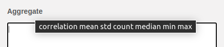
Because rows one and two contain the same values for all of the categorical variables they are aggregated into a single row. By default, the aggregation function is the mean (the 0.5 in the table above is the mean of the two rows that have the same categorical variables), however, you can define other functions. Currently, the available functions are correlation, mean, std, count, median, min and max. You can see the current list of functions by hovering over the Aggregate label.
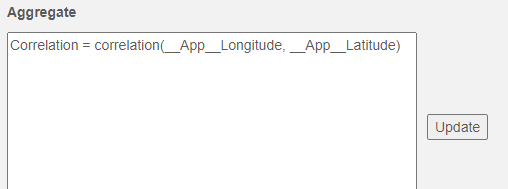
As in the example of correlation, these functions can accept multiple variables. For instance, let's suppose that we were interested in how the latitudes and longitudes for individuals are typically correlated.
We could define Correlation as follows:
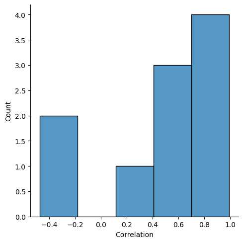
Rows would be grouped by UserId in this case, and the correlation for each participant calculated for the corresponding final table. The histogram for these values looks as follows:
That completes our discussion of the preprocessing capabilities of unforgettable.me. We are expanding the functions from which you can choose rapidly, so be sure to hover over the Compute and Aggregate labels if you are looking for a function that has not been included in this tutorial.
Family = __SEMAg5zn5ggo_B__PeoplePreviousEvent1
Friends = __SEMAg5zn5ggo_B__PeoplePreviousEvent2
Colleagues = __SEMAg5zn5ggo_B__PeoplePreviousEvent3
Classmates = __SEMAg5zn5ggo_B__PeoplePreviousEvent4
Strangers = __SEMAg5zn5ggo_B__PeoplePreviousEvent5
Crowds = __SEMAg5zn5ggo_B__PeoplePreviousEvent6
Alone = __SEMAg5zn5ggo_B__PeoplePreviousEvent7
Pets = __SEMAg5zn5ggo_B__PeoplePreviousEvent8
OtherPeople = __SEMAg5zn5ggo_B__PeoplePreviousEvent9
Partner = __SEMAg5zn5ggo_B__PeoplePreviousEvent10
TV = __SEMAg5zn5ggo_B__ActivitiesPreviousEvent1
Exercising = __SEMAg5zn5ggo_B__ActivitiesPreviousEvent2
Reading = __SEMAg5zn5ggo_B__ActivitiesPreviousEvent3
Eating = __SEMAg5zn5ggo_B__ActivitiesPreviousEvent4
NonDeskWork = __SEMAg5zn5ggo_B__ActivitiesPreviousEvent5
Work = __SEMAg5zn5ggo_B__ActivitiesPreviousEvent6
Meeting = __SEMAg5zn5ggo_B__ActivitiesPreviousEvent7
Chores = __SEMAg5zn5ggo_B__ActivitiesPreviousEvent8
Transit = __SEMAg5zn5ggo_B__ActivitiesPreviousEvent9
Shopping = __SEMAg5zn5ggo_B__ActivitiesPreviousEvent10
SocialMedia = __SEMAg5zn5ggo_B__ActivitiesPreviousEvent11
PrayingMeditating = __SEMAg5zn5ggo_B__ActivitiesPreviousEvent12
Sleeping = __SEMAg5zn5ggo_B__ActivitiesPreviousEvent13
OtherActivity = __SEMAg5zn5ggo_B__ActivitiesPreviousEvent14
Grooming = __SEMAg5zn5ggo_B__ActivitiesPreviousEvent15
[1] Note __SEMAg5zn5ggo_B__PeoplePreviousEvent1 is the variable corresponding to whether the participant indicated that they were with their family when they were notified by SEMA3 in this experiment. Appendix A provides a data dictionary of the people variables and Appendix B a data dictionary of the activity variables.